Threads in operating system
A thread is a single sequence stream within a process. Threads are also called lightweight processes as they possess some of the properties of processes. Each thread belongs to exactly one process.

Thread in Operating System:
- In an operating system that supports multithreading, the process can consist of many threads. But threads can be effective only if the CPU is more than 1 otherwise two threads have to context switch for that single CPU.
- All threads belonging to the same process share – code section, data section, and OS resources (e.g. open files and signals)
- But each thread has its own (thread control block) – thread ID, program counter, register set, and a stack
- Any operating system process can execute a thread. we can say that single process can have multiple threads.
Components of Threads
These are the basic components of the Operating System.
- Stack Space: Stores local variables, function calls, and return addresses specific to the thread.
- Register Set: Hold temporary data and intermediate results for the thread’s execution.
- Program Counter: Tracks the current instruction being executed by the thread.
Types of Thread in Operating System
Threads are of two types. These are described below.
- User Level Thread
- Kernel Level Thread

Threads
1. User Level Thread
User Level Thread is a type of thread that is not created using system calls. The kernel has no work in the management of user-level threads. User-level threads can be easily implemented by the user. In case when user-level threads are single-handed processes, kernel-level thread manages them. Let’s look at the advantages and disadvantages of User-Level Thread.
2. Kernel Level Threads
A kernel Level Thread is a type of thread that can recognize the Operating system easily. Kernel Level Threads has its own thread table where it keeps track of the system. The operating System Kernel helps in managing threads. Kernel Threads have somehow longer context switching time. Kernel helps in the management of threads.
CPU Scheduling in Operating Systems:
CPU scheduling is a process used by the operating system to decide which task or process gets to use the CPU at a particular time. This is important because a CPU can only handle one task at a time, but there are usually many tasks that need to be processed. The following are different purposes of a CPU scheduling time.
- Maximize the CPU utilization
- Minimize the response and waiting time of the process.
What is the Need for a CPU Scheduling Algorithm?
CPU scheduling is the process of deciding which process will own the CPU to use while another process is suspended. The main function of CPU scheduling is to ensure that whenever the CPU remains idle, the OS has at least selected one of the processes available in the ready-to-use line.
In Multiprogramming, if the long-term scheduler selects multiple I/O binding processes then most of the time, the CPU remains idle. The function of an effective program is to improve resource utilization.
Terminologies Used in CPU Scheduling
- Arrival Time: The time at which the process arrives in the ready queue.
- Completion Time: The time at which the process completes its execution.
- Burst Time: Time required by a process for CPU execution.
- Turn Around Time: Time Difference between completion time and arrival time.
Turn Around Time = Completion Time – Arrival Time
- Waiting Time(W.T): Time Difference between turn around time and burst time.
Waiting Time = Turn Around Time – Burst Time
Fixed (or static) Partitioning in Operating System:
Fixed partitioning, also known as static partitioning, is one of the earliest memory management techniques used in operating systems. In this method, the main memory is divided into a fixed number of partitions at system startup, and each partition is allocated to a process. These partitions remain unchanged throughout system operation, ensuring a simple, predictable memory allocation process. Despite its simplicity, fixed partitioning has several limitations, such as internal fragmentation and inflexible handling of varying process sizes. This article delves into the advantages, disadvantages, and applications of fixed partitioning in modern operating systems.
What is Fixed (or static) Partitioning in the Operating System?
Fixed (or static) partitioning is one of the earliest and simplest memory management techniques used in operating systems. It involves dividing the main memory into a fixed number of partitions at system startup, with each partition being assigned to a process. These partitions remain unchanged throughout the system’s operation, providing each process with a designated memory space. This method was widely used in early operating systems and remains relevant in specific contexts like embedded systems and real-time applications. However, while fixed partitioning is simple to implement, it has significant limitations, including inefficiencies caused by internal fragmentation.
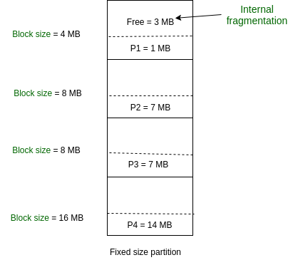
Fixed Partitioning:
This is the oldest and simplest technique used to put more than one process in the main memory. In this partitioning, the number of partitions (non-overlapping) in RAM is fixed but the size of each partition may or may not be the same. As it is a contiguous allocation, hence no spanning is allowed. Here partitions are made before execution or during system configure.
Variable (or Dynamic) Partitioning in Operating System:
Below are Memory Management Techniques.
- Contiguous
- Non-Contiguous
In the Contiguous Technique, the executing process must be loaded entirely in the main memory. The contiguous Technique can be divided into:
- Fixed (static) partitioning
- Variable (dynamic) partitioning
What is Variable (Dynamic) Partitioning?
It is a part of the Contiguous allocation technique. It is used to alleviate the problem faced by Fixed Partitioning. In contrast with fixed partitioning, partitions are not made before the execution or during system configuration. Various features associated with variable Partitioning-
- Initially, RAM is empty and partitions are made during the run-time according to the process’s need instead of partitioning during system configuration.
- The size of the partition will be equal to the incoming process.
- The partition size varies according to the need of the process so that internal fragmentation can be avoided to ensure efficient utilization of RAM.
- The number of partitions in RAM is not fixed and depends on the number of incoming processes and the Main Memory’s size.

Contiguous Memory Allocation:
In contiguous memory allocation, each process is assigned a single continuous block of memory in the main memory. The entire process is loaded into one contiguous memory region.
In Contiguous Technique, executing process must be loaded entirely in the main memory.
Non-Contiguous Memory Allocation:
In non-contiguous memory allocation, a process is divided into multiple blocks or segments that can be loaded into different parts of the memory, rather than requiring a single continuous block.
Virtual Memory in Operating System:
Virtual memory is a memory management technique used by operating systems to give the appearance of a large, continuous block of memory to applications, even if the physical memory (RAM) is limited. It allows larger applications to run on systems with less RAM.
- The main objective of virtual memory is to support multiprogramming, The main advantage that virtual memory provides is, a running process does not need to be entirely in memory.
- Programs can be larger than the available physical memory. Virtual Memory provides an abstraction of main memory, eliminating concerns about storage limitations.
- A memory hierarchy, consisting of a computer system’s memory and a disk, enables a process to operate with only some portions of its address space in RAM to allow more processes to be in memory.
Page Replacement Algorithms in Operating System:
In an operating system that uses paging for memory management, a page replacement algorithm is needed to decide which page needs to be replaced when a new page comes in. Page replacement becomes necessary when a page fault occurs and no free page frames are in memory. in this article, we will discuss different types of page replacement algorithms.
Page Replacement Algorithms
Page replacement algorithms are techniques used in operating systems to manage memory efficiently when the physical memory is full. When a new page needs to be loaded into physical memory, and there is no free space, these algorithms determine which existing page to replace.
If no page frame is free, the virtual memory manager performs a page replacement operation to replace one of the pages existing in memory with the page whose reference caused the page fault. It is performed as follows: The virtual memory manager uses a page replacement algorithm to select one of the pages currently in memory for replacement, accesses the page table entry of the selected page to mark it as “not present” in memory, and initiates a page-out operation for it if the modified bit of its page table entry indicates that it is a dirty page.
Common Page Replacement Techniques
- First In First Out (FIFO)
- Optimal Page replacement
- Least Recently Used (LRU)
- Most Recently Used (MRU)
1. First In First Out (FIFO):
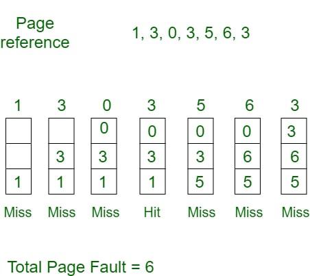
This is the simplest page replacement algorithm. In this algorithm, the operating system keeps track of all pages in the memory in a queue, the oldest page is in the front of the queue. When a page needs to be replaced page in the front of the queue is selected for removal.
Example 1: Consider page reference string 1, 3, 0, 3, 5, 6, 3 with 3-page frames. Find the number of page faults using FIFO Page Replacement Algorithm.
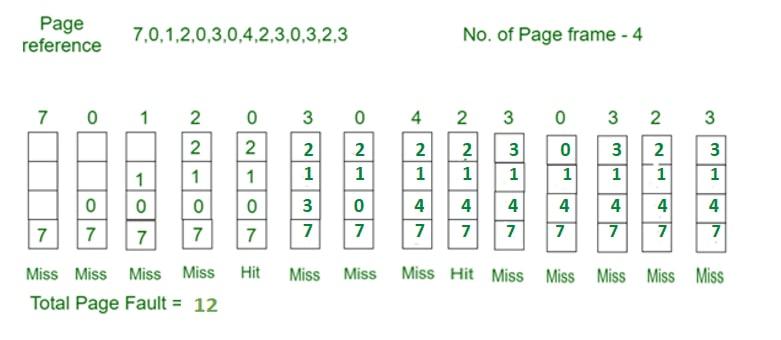
2. Optimal Page Replacement
In this algorithm, pages are replaced which would not be used for the longest duration of time in the future.
Example: Consider the page references 7, 0, 1, 2, 0, 3, 0, 4, 2, 3, 0, 3, 2, 3 with 4-page frame. Find number of page fault using Optimal Page Replacement Algorithm.

3. Least Recently Used:
In this algorithm, page will be replaced which is least recently used.
4. Most Recently Used (MRU):
In this algorithm, page will be replaced which has been used recently. Belady’s anomaly can occur in this algorithm.
Example 4: Consider the page reference string 7, 0, 1, 2, 0, 3, 0, 4, 2, 3, 0, 3, 2, 3 with 4-page frames. Find number of page faults using MRU Page Replacement Algorithm.
Storage Management:
Storage Management is defined as it refers to the management of the data storage equipment’s that are used to store the user/computer generated data. Hence it is a tool or set of processes used by an administrator to keep your data and storage equipment’s safe. Storage management is a process for users to optimize the use of storage devices and to protect the integrity of data for any media on which it resides and the category of storage management generally contain the different type of subcategories covering aspects such as security, virtualization and more, as well as different types of provisioning or automation, which is generally made up the entire storage management software market.
Storage management key attributes: Storage management has some key attribute which is generally used to manage the storage capacity of the system. These are given below:
1. Performance
2. Reliability
3. Recoverability
4. Capacity
File Systems in Operating System:
File systems are a crucial part of any operating system, providing a structured way to store, organize, and manage data on storage devices such as hard drives, SSDs, and USB drives. Essentially, a file system acts as a bridge between the operating system and the physical storage hardware, allowing users and applications to create, read, update, and delete files in an organized and efficient manner.
What is a File System?
A file system is a method an operating system uses to store, organize, and manage files and directories on a storage device. Some common types of file systems include:
- FAT (File Allocation Table): An older file system used by older versions of Windows and other operating systems.
- NTFS (New Technology File System): A modern file system used by Windows. It supports features such as file and folder permissions, compression, and encryption.
- HFS (Hierarchical File System): A file system used by macOS.
- APFS (Apple File System): A new file system introduced by Apple for their Macs and iOS devices
Disk Scheduling Algorithms:
Disk scheduling algorithms are crucial in managing how data is read from and written to a computer’s hard disk. These algorithms help determine the order in which disk read and write requests are processed, significantly impacting the speed and efficiency of data access. Common disk scheduling methods include First-Come, First-Served (FCFS), Shortest Seek Time First (SSTF), SCAN, C-SCAN, LOOK, and C-LOOK. By understanding and implementing these algorithms, we can optimize system performance and ensure faster data retrieval.
- Disk scheduling is a technique operating systems use to manage the order in which disk I/O (input/output) requests are processed.
- Disk scheduling is also known as I/O Scheduling.
- The main goals of disk scheduling are to optimize the performance of disk operations, reduce the time it takes to access data and improve overall system efficiency.
Importance of Disk Scheduling in Operating System
- Multiple I/O requests may arrive by different processes and only one I/O request can be served at a time by the disk controller. Thus other I/O requests need to wait in the waiting queue and need to be scheduled.
- Two or more requests may be far from each other so this can result in greater disk arm movement.
- Hard drives are one of the slowest parts of the computer system and thus need to be accessed in an efficient manner.
Key Terms Associated with Disk Scheduling
- Seek Time: Seek time is the time taken to locate the disk arm to a specified track where the data is to be read or written. So the disk scheduling algorithm that gives a minimum average seek time is better.
- Rotational Latency: Rotational Latency is the time taken by the desired sector of the disk to rotate into a position so that it can access the read/write heads. So the disk scheduling algorithm that gives minimum rotational latency is better.
- Transfer Time: Transfer time is the time to transfer the data. It depends on the rotating speed of the disk and the number of bytes to be transferred.
- Disk Access Time:
Disk Access Time = Seek Time + Rotational Latency + Transfer Time
Total Seek Time = Total head Movement * Seek Time
- Disk Response Time: Response Time is the average time spent by a request waiting to perform its I/O operation. The average Response time is the response time of all requests. Variance Response Time is the measure of how individual requests are serviced with respect to average response time. So the disk scheduling algorithm that gives minimum variance response time is better.
Disk Scheduling Algorithms
There are several Disk Several Algorithms. We will discuss in detail each one of them.
- FCFS (First Come First Serve)
- SSTF (Shortest Seek Time First)
- SCAN
- C-SCAN
- LOOK
- C-LOOK
- RSS (Random Scheduling)
- LIFO (Last-In First-Out)
- N-STEP SCAN
- F-SCAN
1. FCFS (First Come First Serve)
FCFS is the simplest of all Disk Scheduling Algorithms. In FCFS, the requests are addressed in the order they arrive in the disk queue. Let us understand this with the help of an example.
First Come First Serve
Example:
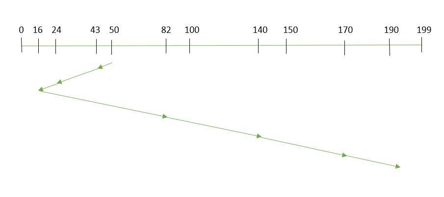
Suppose the order of request is- (82,170,43,140,24,16,190)
And current position of Read/Write head is: 50
So, total overhead movement  (total distance covered by the disk arm) =
(82-50)+(170-82)+(170-43)+(140-43)+(140-24)+(24-16)+(190-16) =642
Advantages of FCFS
Here are some of the advantages of First Come First Serve.
- Every request gets a fair chance
- No indefinite postponement
Disadvantages of FCFS
Here are some of the disadvantages of First Come First Serve.
- Does not try to optimize seek time
- May not provide the best possible service
2. SSTF (Shortest Seek Time First)
In SSTF (Shortest Seek Time First), requests having the shortest seek time are executed first. So, the seek time of every request is calculated in advance in the queue and then they are scheduled according to their calculated seek time. As a result, the request near the disk arm will get executed first. SSTF is certainly an improvement over FCFS as it decreases the average response time and increases the throughput of the system. Let us understand this with the help of an example.
Example:
Shortest Seek Time First
Suppose the order of request is- (82,170,43,140,24,16,190)
And current position of Read/Write head is: 50
So,
total overhead movement  (total distance covered by the disk arm) =
(50-43)+(43-24)+(24-16)+(82-16)+(140-82)+(170-140)+(190-170) =208
Advantages of Shortest Seek Time First
Here are some of the advantages of Shortest Seek Time First.
- The average Response Time decreases
- Throughput increases
Disadvantages of Shortest Seek Time First
Here are some of the disadvantages of Shortest Seek Time First.
- Overhead to calculate seek time in advance
- Can cause Starvation for a request if it has a higher seek time as compared to incoming requests
- The high variance of response time as SSTF favors only some requests
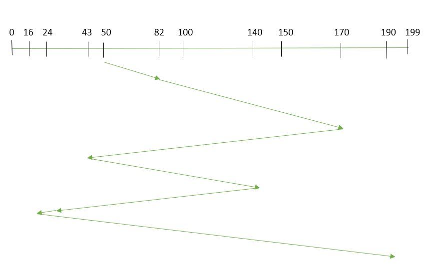
3. SCAN
In the SCAN algorithm the disk arm moves in a particular direction and services the requests coming in its path and after reaching the end of the disk, it reverses its direction and again services the request arriving in its path. So, this algorithm works as an elevator and is hence also known as an elevator algorithm. As a result, the requests at the midrange are serviced more and those arriving behind the disk arm will have to wait.
Example:
SCAN Algorithm
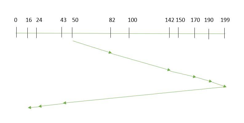
Suppose the requests to be addressed are-82,170,43,140,24,16,190. And the Read/Write arm is at 50, and it is also given that the disk arm should move “towards the larger value”.
Therefore, the total overhead movement (total distance covered by the disk arm) is calculated as
= (199-50) + (199-16) = 332
Advantages of SCAN Algorithm
Here are some of the advantages of the SCAN Algorithm.
- High throughput
- Low variance of response time
- Average response time
Disadvantages of SCAN Algorithm
Here are some of the disadvantages of the SCAN Algorithm.
- Long waiting time for requests for locations just visited by disk arm
4. C-SCAN
In the SCAN algorithm, the disk arm again scans the path that has been scanned, after reversing its direction. So, it may be possible that too many requests are waiting at the other end or there may be zero or few requests pending at the scanned area.
These situations are avoided in the CSCAN algorithm in which the disk arm instead of reversing its direction goes to the other end of the disk and starts servicing the requests from there. So, the disk arm moves in a circular fashion and this algorithm is also similar to the SCAN algorithm hence it is known as C-SCAN (Circular SCAN).
Example:
Circular SCAN
Suppose the requests to be addressed are-82,170,43,140,24,16,190. And the Read/Write arm is at 50, and it is also given that the disk arm should move “towards the larger value”.
So, the total overhead movement (total distance covered by the disk arm) is calculated as:
=(199-50) + (199-0) + (43-0) = 391
Advantages of C-SCAN Algorithm
Here are some of the advantages of C-SCAN.
- Provides more uniform wait time compared to SCAN.
5. LOOK
LOOK Algorithm is similar to the SCAN disk scheduling algorithm except for the difference that the disk arm in spite of going to the end of the disk goes only to the last request to be serviced in front of the head and then reverses its direction from there only. Thus it prevents the extra delay which occurred due to unnecessary traversal to the end of the disk.
Example:

LOOK Algorithm
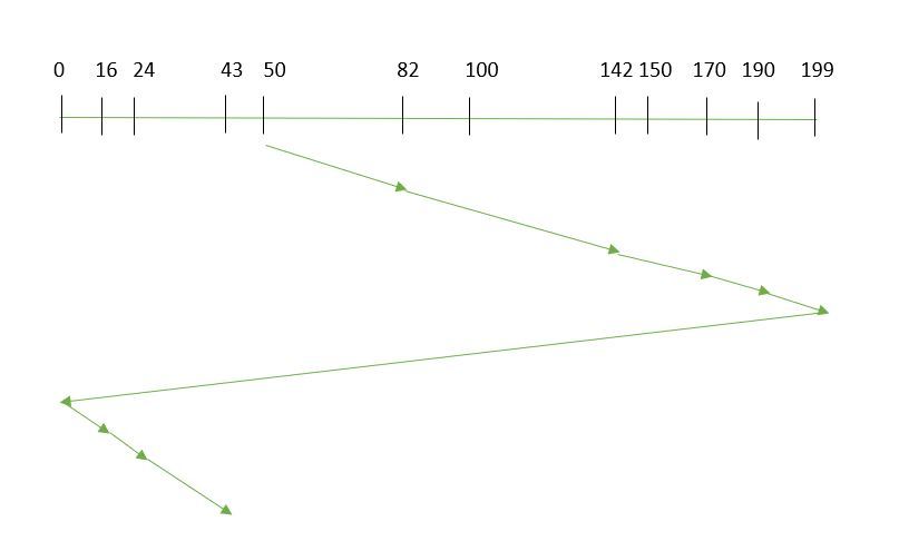
Suppose the requests to be addressed are-82,170,43,140,24,16,190. And the Read/Write arm is at 50, and it is also given that the disk arm should move “towards the larger value”.
So, the total overhead movement (total distance covered by the disk arm) is calculated as:
= (190-50) + (190-16) = 314
6. C-LOOK
As LOOK is similar to the SCAN algorithm, in a similar way, C-LOOK is similar to the CSCAN disk scheduling algorithm. In CLOOK, the disk arm in spite of going to the end goes only to the last request to be serviced in front of the head and then from there goes to the other end’s last request. Thus, it also prevents the extra delay which occurred due to unnecessary traversal to the end of the disk.
Example:
- Suppose the requests to be addressed are-82,170,43,140,24,16,190. And the Read/Write arm is at 50, and it is also given that the disk arm should move “towards the larger value”

C-LOOK
So, the total overhead movement (total distance covered by the disk arm) is calculated as
= (190-50) + (190-16) + (43-16) = 341
7. RSS (Random Scheduling)
It stands for Random Scheduling and just like its name it is natural. It is used in situations where scheduling involves random attributes such as random processing time, random due dates, random weights, and stochastic machine breakdowns this algorithm sits perfectly. Which is why it is usually used for analysis and simulation.
8. LIFO (Last-In First-Out)
In LIFO (Last In, First Out) algorithm, the newest jobs are serviced before the existing ones i.e. in order of requests that get serviced the job that is newest or last entered is serviced first, and then the rest in the same order.
Advantages of LIFO (Last-In First-Out)
Here are some of the advantages of the Last In First Out Algorithm.
- Maximizes locality and resource utilization
- Can seem a little unfair to other requests and if new requests keep coming in, it cause starvation to the old and existing ones.
9. N-STEP SCAN
It is also known as the N-STEP LOOK algorithm. In this, a buffer is created for N requests. All requests belonging to a buffer will be serviced in one go. Also once the buffer is full no new requests are kept in this buffer and are sent to another one. Now, when these N requests are serviced, the time comes for another top N request and this way all get requests to get a guaranteed service
Advantages of N-STEP SCAN
Here are some of the advantages of the N-Step Algorithm.
- It eliminates the starvation of requests completely
10. F-SCAN
This algorithm uses two sub-queues. During the scan, all requests in the first queue are serviced and the new incoming requests are added to the second queue. All new requests are kept on halt until the existing requests in the first queue are serviced.
RAID (Redundant Arrays of Independent Disks)
RAID (Redundant Arrays of Independent Disks) is a technique that makes use of a combination of multiple disks for storing the data instead of using a single disk for increased performance, data redundancy, or to protect data in the case of a drive failure. The term was defined by David Patterson, Garth A. Gibson, and Randy Katz at the University of California, Berkeley in 1987. In this article, we are going to discuss RAID and types of RAID their Advantages and disadvantages in detail.
What is RAID?
RAID (Redundant Array of Independent Disks) is like having backup copies of your important files stored in different places on several hard drives or solid-state drives (SSDs). If one drive stops working, your data is still safe because you have other copies stored on the other drives. It’s like having a safety net to protect your files from being lost if one of your drives breaks down.
RAID (Redundant Array of Independent Disks) in a Database Management System (DBMS) is a technology that combines multiple physical disk drives into a single logical unit for data storage. The main purpose of RAID is to improve data reliability, availability, and performance. There are different levels of RAID, each offering a balance of these benefits.
Why Data Redundancy?
Data redundancy, although taking up extra space, adds to disk reliability. This means, that in case of disk failure, if the same data is also backed up onto another disk, we can retrieve the data and go on with the operation. On the other hand, if the data is spread across multiple disks without the RAID technique, the loss of a single disk can affect the entire data.
Key Evaluation Points for a RAID System :
When evaluating a RAID system, the following critical aspects should be considered:
1. Reliability
Definition: Refers to the system’s ability to tolerate disk faults and prevent data loss.
Key Questions:
- How many disk failures can the RAID configuration sustain without losing data?
- Is there redundancy in the system, and how is it implemented (e.g., parity, mirroring)?
Example:
- RAID 0 offers no fault tolerance; if one disk fails all data is lost.
- RAID 5 can tolerate one disk failure due to parity data.
- RAID 6 can handle two simultaneous disk failures.
2. Availability
Definition: The fraction of time the RAID system is operational and available for use.
Key Questions:
- What is the system’s uptime, and how quickly can it recover from failures?
- Can data be accessed during disk rebuilds or replacements?
Example:
- RAID 1 (Mirroring) allows immediate data access even during a single disk failure.
- RAID 5 and 6 may degrade performance during a rebuild, but data remains available.
3. Performance
Definition: Measures how efficiently the RAID system handles data processing tasks. This includes:
- Response Time: How quickly the system responds to data requests.
- Throughput: The rate at which the system processes data (e.g., MB/s or IOPS).
Key Factors:
- RAID levels affect performance differently:
- RAID 0 offers high throughput but no redundancy.
- RAID 1 improves read performance by serving data from either mirrored disk but may not improve write performance significantly.
- RAID 5/6 introduces overhead for parity calculations, affecting write speeds.
- Workload type (e.g., sequential vs. random read/write operations).
Performance Trade-offs: Higher redundancy often comes at the cost of slower writes (due to parity calculations).
4. Capacity
Definition: The amount of usable storage available to the user after accounting for redundancy mechanisms.
Key Calculation: For a set of N disks, each with B blocks, the available capacity depends on the RAID level:
- RAID 0: All N×B blocks are usable (no redundancy).
- RAID 1: Usable capacity is B (only one disk’s capacity due to mirroring).
- RAID 5: Usable capacity is (N−1)×B (one disk’s worth of capacity used for parity).
- RAID 6: Usable capacity is (N−2)×B (two disks’ worth used for parity).