INTRODUCTION TO THEORY OF COMPUTATION

• Automata theory, also known as the Theory of Computation, is a field within computer science and mathematics that focuses on studying abstract machines to understand the capabilities and limitations of computation by analyzing mathematical models of how machines can perform calculations.
• The main motivation behind developing Automata Theory was to develop methods to describe and analyze the dynamic behavior of discrete systems.

• Theory of Computation is divided into three main areas:

  • Automata Theory: Studies abstract machines and formal languages, which are crucial for compiler design, natural language processing (NLP), and pattern recognition.
  • Computability Theory: Explores which problems can be solved by a computer and helps in understanding undecidable problems and recursive functions.
  • Complexity Theory: Analyzes how efficiently a problem can be solved, classifying problems into categories like P, NP, and NP-complete to optimize algorithm performance.

BASIC TERMINOLOGIES:

• Now, let’s understand the basic terminologies, which are important and frequently used in the Theory of Computation. 

  1. Symbol

• A symbol (often also called a character) is the smallest building block, which can be any alphabet, letter, or picture. 

  2. Alphabets (Σ)

• A finite, non-empty set of symbols used to construct strings and languages. 
• Alphabets are a set of symbols, which are always finite.

  3. String

• A string is a finite sequence of symbols from some alphabet. A string is generally denoted as w and the length of a string is denoted as |w|. Empty string is the string with zero occurrence of symbols, represented as ε.

   

  Number of Strings (of length 2)
  that can be generated over the alphabet {a, b}:
  – –
  a a
  a b
  b a
  b b
  
  Length of String |w| = 2
  Number of Strings = 4
  
  Conclusion:
  For alphabet {a, b} with length n, number of
  strings can be generated = 2ⁿ.

AUTOMATA

• Automata Theory is a branch of the Theory of Computation. It deals with the study of abstract machines and their capacities for computation.
• An abstract machine is called the automata. It includes the design and analysis of automata, which are mathematical models that can perform computations on strings of symbols according to a set of rules.

• Automata Theory has far-reaching applications in a variety of fields. Understanding these applications can give us insights into how powerful and versatile this branch of computer science is:

  • Compiler Design: Automata are essential for parsing programming languages and converting source code into machine-readable instructions.
  • Natural Language Processing (NLP): Automata play a key role in processing human language. In speech recognition, chatbots, and text analysis, automata are used to recognize patterns in language and structure sentences for machine understanding.
  • Pattern Recognition: Automata are used in image processing, handwriting recognition, and bioinformatics to detect patterns and match specific data structures. They help in recognizing objects in images, fingerprints, and even genetic patterns.
  • Search Engines & Data Validation: Regular expressions, a simplified form of finite automata, are extensively used in search engines, data validation, and filtering. These tools help match patterns in large datasets and validate inputs in forms or databases.
  • Cybersecurity: Automata are used in intrusion detection systems and malware detection. By recognizing malicious patterns in network traffic or files, automata help protect systems from security breaches and cyberattacks.
  • AI & Machine Learning: Automata models are used in AI applications to process and recognize sequences of events, helping train models for applications like speech synthesis, image classification, and pattern prediction.

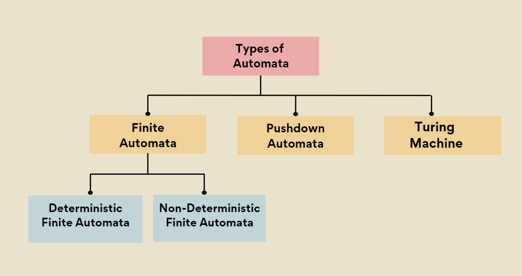
TYPES OF AUTOMATA:

FINITE AUTOMATA:

• Finite automata are abstract machines used to recognize patterns in input sequences, forming the basis for understanding regular languages in computer science. They consist of states, transitions, and input symbols, processing each symbol step-by-step.

• Features of Finite Automata:

  • Input: Set of symbols or characters provided to the machine.
  • Output: Accept or reject based on the input pattern.
  • States of Automata: The conditions or configurations of the machine.
  • State Relation: The transitions between states.
  • Output Relation: Based on the final state, the output decision is made.

• A finite automaton can be defined as a tuple:

  { Q, Σ, q, F, δ }, where:

  • Q: Finite set of states
  • Σ: Set of input symbols
  • q: Initial state
  • F: Set of final states
  • δ: Transition function

• There are two types of finite automata:

  • Deterministic Fintie Automata (DFA)
  • Non-Deterministic Finite Automata (NFA)

DETERMINISTIC FINITE AUTOMATA (DFA):

• A DFA is represented as {Q, Σ, q, F, δ}. In DFA, for each input symbol, the machine transitions to one and only one state. DFA does not allow any null transitions, meaning every state must have a transition defined for every input symbol.

• Construct a DFA that accepts all strings ending with ‘a’.

  Given:

  Σ = {a, b},

  Q = {q0, q1},

  F = {q1}

  
  

  State/Symbol	a	b
  q0	q1	q0
  q1	q1	q0

  In this example, if the string ends in ‘a’, the machine reaches state q1, which is an accepting state.

NON-DETERMINISTIC FINITE AUTOMATA (NFA):

• NFA is similar to DFA but includes the following features:

  • It can transition to multiple states for the same input.
  • It allows null (ϵ) moves, where the machine can change states without consuming any input.

• Construct an NFA that accepts strings ending in ‘a’.

  Given:

  Σ = {a, b},

  Q = {q0, q1},

  F = {q1}

  
  

  State Transition Table for above Automaton,

  State/Symbol	a	b
  q0	{q0,q1}	q0
  q1	φ	φ

  In an NFA, if any transition leads to an accepting state, the string is accepted.

• Although NFAs appear more flexible, they do not have more computational power than DFAs. Every NFA can be converted to an equivalent DFA, although the resulting DFA may have more states.

  • DFA: Single transition for each input symbol, no null moves.
  • NFA: Multiple transitions and null moves allowed.
  • Power: Both DFA and NFA recognize the same set of regular languages.

CONVERSION FROM NFA TO DFA:

• An NFA can have zero, one or more than one move from a given state on a given input symbol. An NFA can also have NULL moves (moves without input symbol). On the other hand, DFA has one and only one move from a given state on a given input symbol. 
• To convert the NFA to its equivalent transition table, we need to list all the states, input symbols, and the transition rules.
• The DFA’s start state is the set of all possible starting states in the NFA. This set is called the “epsilon closure” of the NFA’s start state. The epsilon closure is the set of all states that can be reached from the start state by following epsilon (?) transitions.
• The DFA’s final states are the sets of states that contain at least one final state from the NFA.

• The DFA obtained in the previous steps may contain unnecessary states and transitions. To simplify the DFA, we can use the following techniques:

  • Remove unreachable states: States that cannot be reached from the start state can be removed from the DFA.
  • Remove dead states: States that cannot lead to a final state can be removed from the DFA.
  • Merge equivalent states: States that have the same transition rules for all input symbols can be merged into a single state.
• After simplifying the DFA, we repeat steps 3-5 until no further simplification is possible. The final DFA obtained is the minimized DFA equivalent to the given NFA.
• Example: Consider the following NFA:

Following are the various parameters for NFA. Q = { q0, q1, q2 } ? = ( a, b ) F = { q2 } ? (Transition Function of NFA) :

The final DFA for above NFA will be :

PUSH-DOWN AUTOMATA:

• Pushdown Automata is a finite automata with extra memory called stack which helps Pushdown automata to recognize Context Free Languages. 

• A Pushdown Automata (PDA) can be defined as : 

  • Q is the set of states
  • ∑is the set of input symbols
  • Γ is the set of pushdown symbols (which can be pushed and popped from the stack)
  • q0 is the initial state
  • Z is the initial pushdown symbol (which is initially present in the stack)
  • F is the set of final states
  • δ is a transition function that maps Q x {Σ ∪ ∈} x Γ into Q x Γ*. In a given state, the PDA will read the input symbol and stack symbol (top of the stack) move to a new state, and change the symbol of the stack.

• Instantaneous Description (ID) is an informal notation of how a PDA “computes” an input string and makes a decision whether that string is accepted or rejected. 

  An ID is a triple (q, w, α), where: 
  1. q is the current state. 
  2. w is the remaining input. 
  3.α is the stack contents, top at the left. 

• Example : Define the pushdown automata for language {aⁿbⁿ | n > 0} 
  Solution : M = where Q = { q0, q1 } and Σ = { a, b } and Γ = { A, Z } and δ is given by : 

  δ( q0, a, Z ) = { ( q0, AZ ) } 
  δ( q0, a, A) = { ( q0, AA ) } 
  δ( q0, b, A) = { ( q1, ∈) } 
  δ( q1, b, A) = { ( q1, ∈) } 
  δ( q1, ∈, Z) = { ( q1, ∈) } 

• Explanation : Initially, the state of Automata is q0 and symbol on stack is Z and the input is aaabbb as shown in row 1. On reading ‘a’ (shown in bold in row 2), the state will remain q0 and it will push symbol A on stack. On next ‘a’ (shown in row 3), it will push another symbol A on stack. After reading 3 a’s, the stack will be AAAZ with A on the top. After reading ‘b’ (as shown in row 5), it will pop A and move to state q1 and stack will be AAZ. When all b’s are read, the state will be q1 and stack will be Z. In row 8, on input symbol ‘∈’ and Z on stack, it will pop Z and stack will be empty. This type of acceptance is known as acceptance by empty stack. 

TURING MACHINE:

• Turing Machines (TM) play a crucial role in the Theory of Computation (TOC). They are abstract computational devices used to explore the limits of what can be computed.
• Turing Machines help prove that certain languages and problems have no algorithmic solution. Their simplicity makes them an effective tool for studying computational theory, yet they are as powerful as modern computers.
• Turing Machine was invented by Alan Turing in 1936 and it is used to accept Recursive Enumerable Languages (generated by Type-0 Grammar). 
• A Turing Machine consists of an infinite tape, a read/write head, and a set of rules that determine how it reads, writes, and moves on the tape. Despite its simplicity, a TM can simulate any real-world computation, making it as powerful as modern computers but with infinite memory.

• Turing Machines are preferred because:

  • They are simpler to analyze.
  • They provide a clear, mathematical model of computation.
  • They possess infinite memory, making them even more powerful than real-world computers.

• A Turing Machine is defined by:

  1. A finite set of states (Q).
  2. An input alphabet (Σ).
  3. A tape alphabet (Γ) that includes Σ.
  4. A transition function (δ).
  5. A start state (q0).
  6. A blank symbol (B).
  7. A set of final states (F).

• Example:

  We construct a Turing Machine (TM) for the language L = {0ⁿ1ⁿ | n ≥ 1}, which accepts strings of equal 0s followed by equal 1s.

  Components:

  • Q = {q₀, q₁, q₂, q₃} (q₀ is the initial state)
  • T = {0,1,X,Y,B} (B represents blank, X and Y mark processed symbols)
  • Σ = {0,1} (input symbols)
  • F = {q₃} (final state)

  Transition Table:

  

  Let us see how this turing machine works for 0011. Initially head points to 0 which is underlined and state is q0 as:  

  

  The move will be δ(q0, 0) = (q1, X, R). It means, it will go to state q1, replace 0 by X and head will move to right as:  

  

  The move will be δ(q1, 0) = (q1, 0, R) which means it will remain in same state and without changin any symbol, it will move to right as:  

  

  The move will be δ(q1, 1) = (q2, Y, L) which means it will move to q2 state and changing 1 to Y, it will move to left as:  

  

  Working on it in the same way, the machine will reach state q3 and head will point to B as shown:  

  

  Using move δ(q3, B) = halt, it will stop and accepted.