NEED OF ALGORITHM IN DATA STRUCTURE!

• Algorithm may be defined as "A procedure for solving a mathematical problem in a finite number of steps that frequently involves recursive operations”.

• Algorithms play a crucial role in various fields and have many applications. Some of the key areas where algorithms are used include:

  1. Computer Science: Algorithms form the basis of computer programming and are used to solve problems ranging from simple sorting and searching to complex tasks such as artificial intelligence and machine learning.
  2. Mathematics: Algorithms are used to solve mathematical problems, such as finding the optimal solution to a system of linear equations or finding the shortest path in a graph.
  3. Operations Research: Algorithms are used to optimize and make decisions in fields such as transportation, logistics, and resource allocation.
  4. Artificial Intelligence: Algorithms are the foundation of artificial intelligence and machine learning, and are used to develop intelligent systems that can perform tasks such as image recognition, natural language processing, and decision-making.
  5. Data Science: Algorithms are used to analyze, process, and extract insights from large amounts of data in fields such as marketing, finance, and healthcare.
• Algorithms also enable computers to perform tasks that would be difficult or impossible for humans to do manually.

PROPERTIES:

• It should terminate after a finite time.
• It should produce at least one output.
• It should take zero or more input.
• It should be deterministic means giving the same output for the same input case.
• Every step in the algorithm must be effective i.e. every step should do some work.

APPROACHES OF ALGORITHM

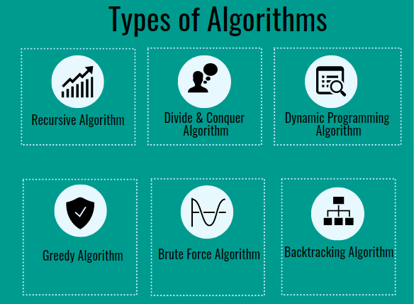
BRUTE FORCE ALGORITHM:

• It is the simplest approach to a problem. A brute force algorithm is the first approach that comes to finding when we see a problem.
• The general logic structure is applied to design an algorithm. It is also known as an exhaustive search algorithm that searches all the possibilities to provide the required solution.

RECURSIVE ALGORITHM:

• A recursive algorithm is based on recursion. In this case, a problem is broken into several sub-parts and called the same function again and again.

SEARCHING ALGORITHM:

• Searching algorithms are the ones that are used for searching elements or groups of elements from a particular data structure. They can be of different types based on their approach or the data structure in which the element should be found.

SORTING ALGORITHM:

• Sorting is arranging a group of data in a particular manner according to the requirement. The algorithms which help in performing this function are called sorting algorithms. Generally sorting algorithms are used to sort groups of data in an increasing or decreasing manner.

HASHING ALGORITHM:

• Hashing algorithms work similarly to the searching algorithm. But they contain an index with a key ID. In hashing, a key is assigned to specific data.

DIVIDE AND CONQUER ALGORITHM:

• This algorithm breaks a problem into sub-problems, solves a single sub-problem, and merges the solutions to get the final solution. It consists of the following three steps:

  • Divide
  • Solve
  • Combine
•  It allows you to break down the problem into different methods, and valid output is produced for the valid input. This valid output is passed to some other function.

GREEDY ALGORITHM:

• In this type of algorithm, the solution is built part by part. The solution for the next part is built based on the immediate benefit of the next part. The one solution that gives the most benefit will be chosen as the solution for the next part.

TYPES OF SORTING ALGORITHM

MERGE SORT:

• Merge sort is a sorting algorithm that follows the divide and conquer approach. It works by recursively dividing the input array into smaller subarrays and sorting those subarrays then merging them back together to obtain the sorted array.
• We can say that the process of merge sort is to divide the array into two halves, sort each half, and then merge the sorted halves back together. This process is repeated until the entire array is sorted.

• Here’s a step-by-step explanation of how merge sort works:

  1. Divide: Divide the list or array recursively into two halves until it can no more be divided.
  2. Conquer: Each subarray is sorted individually using the merge sort algorithm.
  3. Merge: The sorted subarrays are merged back together in sorted order. The process continues until all elements from both subarrays have been merged.

• Time Complexity:
  • Best Case: O(n log n), When the array is already sorted or nearly sorted.
  • Average Case: O(n log n), When the array is randomly ordered.
  • Worst Case: O(n log n), When the array is sorted in reverse order.
• Auxiliary Space: O(n), Additional space is required for the temporary array used during merging.

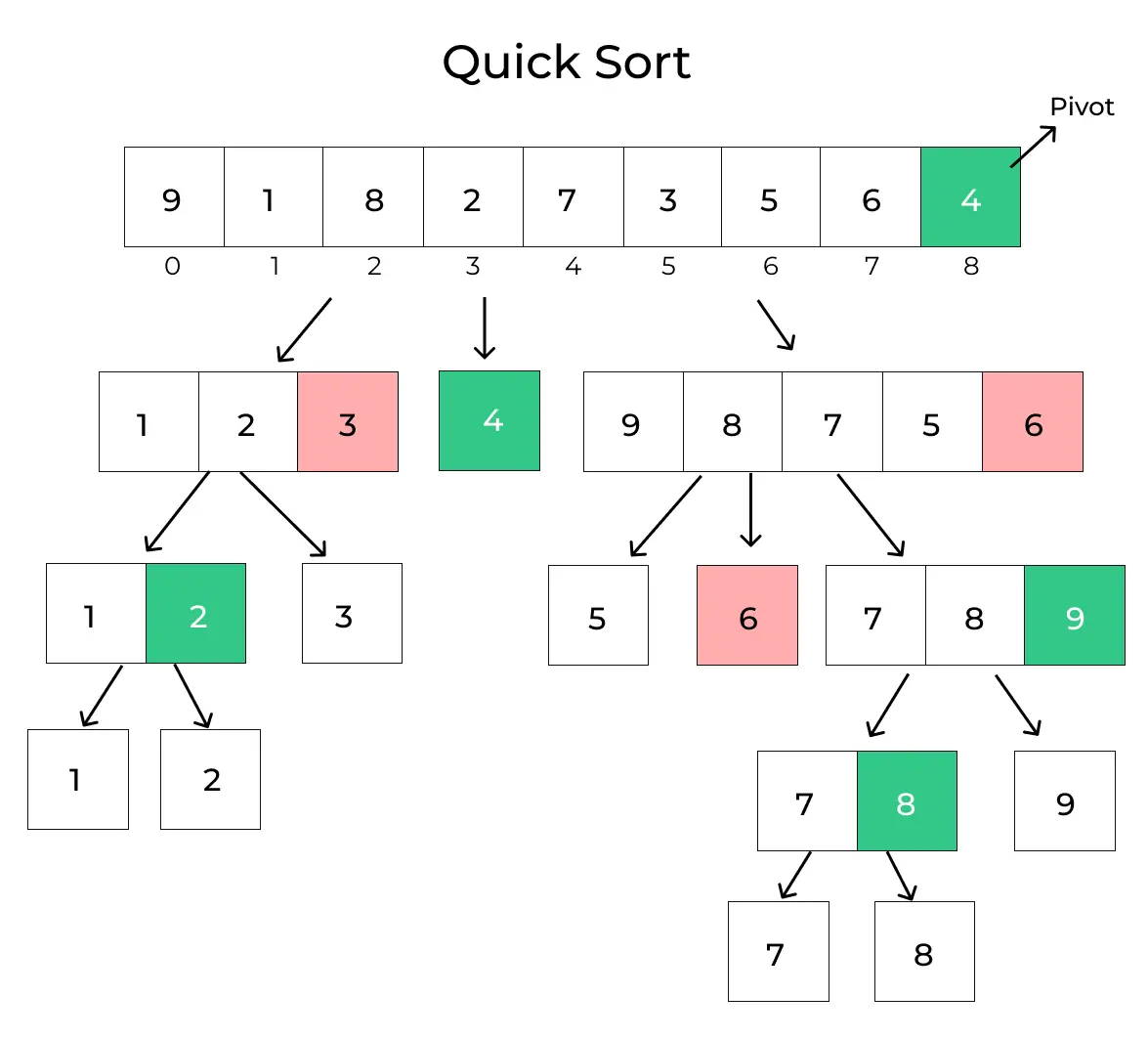
QUICK SORT:

• QuickSort is a sorting algorithm based on the divide and conquer approach that picks an element as a pivot and partitions the given array around the picked pivot by placing the pivot in its correct position in the sorted array.

• There are mainly three steps in this algorithm:

  1. Choose a Pivot: Select an element from the array as the pivot. The choice of pivot can vary (e.g., first element, last element, random element, or median).
  2. Partition the Array: Rearrange the array around the pivot. After partitioning, all elements smaller than the pivot will be on its left, and all elements greater than the pivot will be on its right. The pivot is then in its correct position, and we obtain the index of the pivot.
  3. Recursively Call: Recursively apply the same process to the two partitioned sub-arrays (left and right of the pivot).
  4. Base Case: The recursion stops when there is only one element left in the sub-array, as a single element is already sorted.

• Time Complexity:

  • Best Case: (Ω(n log n)), Occurs when the pivot element divides the array into two equal halves.
  • Average Case (θ(n log n)), On average, the pivot divides the array into two parts, but not necessarily equal.
  • Worst Case: (O(n²)), Occurs when the smallest or largest element is always chosen as the pivot (e.g., sorted arrays).

• Auxiliary Space: O(n), due to recursive call stack.

SELECTION SORT:

• Selection Sort is a comparison-based sorting algorithm. It sorts an array by repeatedly selecting the smallest (or largest) element from the unsorted portion and swapping it with the first unsorted element. This process continues until the entire array is sorted.
• First we find the smallest element and swap it with the first element. This way we get the smallest element at its correct position.
• Then we find the smallest among remaining elements (or second smallest) and swap it with the second element.
• We keep doing this until we get all elements moved to correct position.

• Time Complexity: O(n²) ,as there are two nested loops:

  • One loop to select an element of Array one by one = O(n)
  • Another loop to compare that element with every other Array element = O(n)
  • Therefore overall complexity = O(n) * O(n) = O(n*n) = O(n²)

• Auxiliary Space: O(1) as the only extra memory used is for temporary variables.

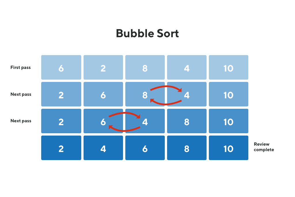
BUBBLE SORT:

• Bubble Sort is the simplest sorting algorithm that works by repeatedly swapping the adjacent elements if they are in the wrong order. This algorithm is not suitable for large data sets as its average and worst-case time complexity are quite high.
• We sort the array using multiple passes. After the first pass, the maximum element goes to end (its correct position). Same way, after second pass, the second largest element goes to second last position and so on.
• In every pass, we process only those elements that have already not moved to correct position. After k passes, the largest k elements must have been moved to the last k positions.
• In a pass, we consider remaining elements and compare all adjacent and swap if larger element is before a smaller element. If we keep doing this, we get the largest (among the remaining elements) at its correct position.
• Time Complexity: O(n²)
  
• Auxiliary Space: O(1)

HEAP SORT:

• Heap sort is a comparison-based sorting technique based on Binary heap data structure. It can be seen as an optimization over selection sort where we first find the max (or min) element and swap it with the last (or first). We repeat the same process for the remaining elements.
• In Heap Sort, we use Binary Heap so that we can quickly find and move the max element in O(Log n) instead of O(n) and hence achieve the O(n Log n) time complexity.

• First convert the array into a max heap using heapify, Please note that this happens in-place. The array elements are re-arranged to follow heap properties. Then one by one delete the root node of the Max-heap and replace it with the last node and heapify. Repeat this process while size of heap is greater than 1.

  • Rearrange array elements so that they form a Max Heap.
  • Repeat the following steps until the heap contains only one element:
    • Swap the root element of the heap (which is the largest element in current heap) with the last element of the heap.
    • Remove the last element of the heap (which is now in the correct position). We mainly reduce heap size and do not remove element from the actual array.
    • Heapify the remaining elements of the heap.
  • Finally we get sorted array.
• Time Complexity: O(n log n)
  
• Auxiliary Space: O(log n), due to the recursive call stack. However, auxiliary space can be O(1) for iterative implementation.

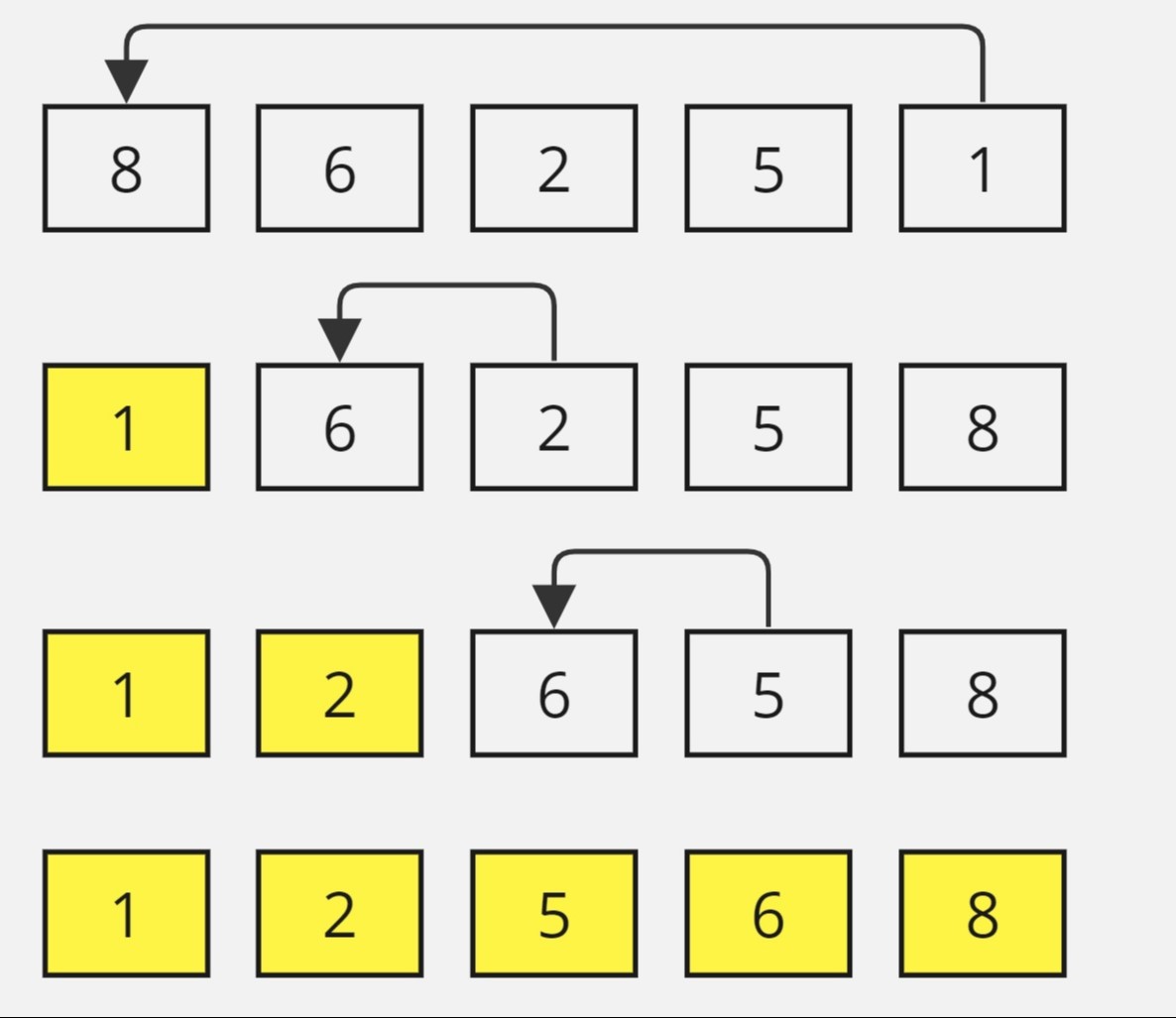
INSERTION SORT:

• Insertion sort is a simple sorting algorithm that works by iteratively inserting each element of an unsorted list into its correct position in a sorted portion of the list.
• It is like sorting playing cards in your hands. You split the cards into two groups: the sorted cards and the unsorted cards. Then, you pick a card from the unsorted group and put it in the right place in the sorted group.
• We start with second element of the array as first element in the array is assumed to be sorted.
• Compare second element with the first element and check if the second element is smaller then swap them.
• Move to the third element and compare it with the first two elements and put at its correct position
• Repeat until the entire array is sorted.

• Time Complexity:

  • Best case: O(n), If the list is already sorted, where n is the number of elements in the list.
  • Average case: O(n²), If the list is randomly ordered
  • Worst case: O(n²), If the list is in reverse order

• Space Complexity:

  • Auxiliary Space: O(1), Insertion sort requires O(1) additional space, making it a space-efficient sorting algorithm.

COMPARING COMPLEXITY ANALYSIS:

HASHING (HASH FUNCTION)

• Hashing is a technique used in data structures that efficiently stores and retrieves data in a way that allows for quick access.
• Hashing involves mapping data to a specific index in a hash table (an array of items) using a hash function. It enables fast retrieval of information based on its key.
• The great thing about hashing is, we can achieve all three operations (search, insert and delete) in O(1) time on average.
• Hashing is mainly used to implement a set of distinct items (only keys) and dictionaries (key value pairs).

• There are majorly three components of hashing:

  1. Key: A Key can be anything string or integer which is fed as input in the hash function the technique that determines an index or location for storage of an item in a data structure.
  2. Hash Function: Receives the input key and returns the index of an element in an array called a hash table. The index is known as the hash index .
  3. Hash Table: Hash table is typically an array of lists. It stores values corresponding to the keys. Hash stores the data in an associative manner in an array where each data value has its own unique index.

HOW DOES HASHING WORK ?

• Suppose we have a set of strings {“ab”, “cd”, “efg”} and we would like to store it in a table.

  • Step 1: We know that hash functions (which is some mathematical formula) are used to calculate the hash value which acts as the index of the data structure where the value will be stored.
  • Step 2: So, let’s assign
    • “a” = 1,
    • “b”=2, .. etc, to all alphabetical characters.
  • Step 3: Therefore, the numerical value by summation of all characters of the string:

  • “ab” = 1 + 2 = 3,
  • “cd” = 3 + 4 = 7 ,
  • “efg” = 5 + 6 + 7 = 18

  • Step 4: Now, assume that we have a table of size 7 to store these strings. The hash function that is used here is the sum of the characters in key mod Table size . We can compute the location of the string in the array by taking the sum(string) mod 7 .
  • Step 5: So we will then store
    • “ab” in 3 mod 7 = 3,
    • “cd” in 7 mod 7 = 0, and
    • “efg” in 18 mod 7 = 4.

WHAT IS COLLISION IN HASHING ?

• When two or more keys have the same hash value, a collision happens. If we consider the above example, the hash function we used is the sum of the letters, but if we examined the hash function closely then the problem can be easily visualised that for different strings same hash value is being generated by the hash function.
• For example: {“ab”, “ba”} both have the same hash value, and string {“cd”,”be”} also generate the same hash value, etc. This is known as collision and it creates problem in searching, insertion, deletion, and updating of value.
• The probability of a hash collision depends on the size of the algorithm, the distribution of hash values and the efficiency of Hash function. To handle this collision, we use Collision Resolution Techniques.

SEPERATE CHAINING COLLISON IN HASHING

• Separate chaining is one of the most popular and commonly used techniques in order to handle collisions. 

• Advantages:

  • Simple to implement. 
  • Hash table never fills up, we can always add more elements to the chain. 
  • Less sensitive to the hash function or load factors. 
  • It is mostly used when it is unknown how many and how frequently keys may be inserted or deleted. 

• Disadvantages: 

  • The cache performance of chaining is not good as keys are stored using a linked list. Open addressing provides better cache performance as everything is stored in the same table. 
  • Wastage of Space (Some Parts of the hash table are never used) 
  • If the chain becomes long, then search time can become O(n) in the worst case
  • Uses extra space for links

OPEN ADDRESSING COLLISION IN HASHING

• Open Addressing is a method for handling collisions. In Open Addressing, all elements are stored in the hash table itself. So at any point, the size of the table must be greater than or equal to the total number of keys (Note that we can increase table size by copying old data if needed). This approach is also known as closed hashing. This entire procedure is based upon probing.
• Insert(k): Keep probing until an empty slot is found. Once an empty slot is found, insert k. 
• Search(k): Keep probing until the slot’s key doesn’t become equal to k or an empty slot is reached. 
• Delete(k): Delete operation is interesting. If we simply delete a key, then the search may fail. So slots of deleted keys are marked specially as “deleted”. 
  The insert can insert an item in a deleted slot, but the search doesn’t stop at a deleted slot. 

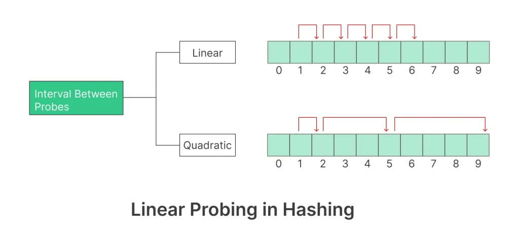
LINEAR PROBING:

• In linear probing, the hash table is searched sequentially that starts from the original location of the hash. If in case the location that we get is already occupied, then we check for the next location. 
• The function used for rehashing is as follows:   rehash(key) = (n+1)%table-size. 

DOUBLE HASHING:

• The intervals that lie between probes are computed by another hash function. Double hashing is a technique that reduces clustering in an optimized way.
• In this technique, the increments for the probing sequence are computed by using another hash function. We use another hash function hash2(x) and look for the i*hash2(x) slot in the i^th rotation. 

QUADRATIC PROBING:

• This method is also known as the mid-square method. In this method, we look for the i²‘th slot in the i^th iteration. We always start from the original hash location. If only the location is occupied then we check the other slots.
• If you observe carefully, then you will understand that the interval between probes will increase proportionally to the hash value. Quadratic probing is a method with the help of which we can solve the problem of clustering that was discussed above. 

COMPARISON OF ABOVE THREE PROBING:

• Open addressing is a collision handling technique used in hashing where, when a collision occurs (i.e., when two or more keys map to the same slot), the algorithm looks for another empty slot in the hash table to store the collided key.
• In linear probing, the algorithm simply looks for the next available slot in the hash table and places the collided key there. If that slot is also occupied, the algorithm continues searching for the next available slot until an empty slot is found. This process is repeated until all collided keys have been stored. Linear probing has the best cache performance but suffers from clustering. One more advantage of Linear probing is easy to compute. 
• In quadratic probing, the algorithm searches for slots in a more spaced-out manner. When a collision occurs, the algorithm looks for the next slot using an equation that involves the original hash value and a quadratic function. If that slot is also occupied, the algorithm increments the value of the quadratic function and tries again. This process is repeated until an empty slot is found. Quadratic probing lies between the two in terms of cache performance and clustering. 
• In double hashing, the algorithm uses a second hash function to determine the next slot to check when a collision occurs. The algorithm calculates a hash value using the original hash function, then uses the second hash function to calculate an offset. The algorithm then checks the slot that is the sum of the original hash value and the offset. If that slot is occupied, the algorithm increments the offset and tries again. This process is repeated until an empty slot is found.  Double hashing has poor cache performance but no clustering. Double hashing requires more computation time as two hash functions need to be computed.